Motive

My motive for interpolation is to implement a simulator for a self-gravitating torus-shaped set of orbit. The torus can be modeled as a set of rings, where all the rings are around a common axis. The problem is symmetric, so I don't have to simulate a thousand points per ring attracting every other point in the simulation, I just have to know the function of how one ring attracts a point on another ring, then I can calculate how the rings attract one another. It turns out there is no closed form for how one ring attracts another, so the best I can do is collect a bunch of sample points and interpolate between them. Since the rings occupy 3-space and can be any size (but are parallel and have a common axis), this is a 2-d function, where you assume the outer ring is at (1,0) and the inner ring is at (x,y) where 0 ≤ x ≤ 1 and y ≥ 0. There's a pole at (1,0), other than that it's smooth and eventually resembles 1/distance² (with an x and y component). X is towards the axis, Y is parallel to the axis, and Z is perpendicular to both and the rings always exert no force on each other in the Z direction.

Lagrange interpolation on equally spaced gridpoints

I have some code for Lagrange interpolation of evenly spaced points. For 2D interpolation, if you need n points, you first do n Lagrange interpolations in the x axis to get consecutive points in the y dimension, then do the same Lagrange interpolation on those interpolated points to get the final answer.

I treated x=0 as happening in the middle of the two middle points, with the given points landing on odd integers, which made the problem symmetric and reduced the number of multiplies needed. Higher-order Lagrange extrapolation (guessing values outside of the given values) rightfully has a bad reputation for being wildly inaccurate, but it does quite well for interpolation between the middle values, provided you make the interval small enough. The number of digits of accuracy increases linearly with the degree of the formula. For example, a 7th degree formula needs 8 support points and requires 41 multiplications, and given a 105-element table of the values of sin(x) at degrees -7 through 97, it can calculate values of sin(x) to 15 or 16 digits accuracy (which is all a double can encode). Below, they are calculating the sine of 44.0, 44.25, 44.5, 44.75, 45 degrees, given the sine of 40, 41, 42, 43, 44, 45, 46, 47, 48, 49 degrees.

C:\bob\cplus\ring>lagrange 0.6427876096865393263226434 0.6560590289905072847824949 0.66913060635885821382627 0.68199836006249850044222578 0.6946583704589972866564 0.70710678118654752440084436 0.71933980033865113935605467 0.7313537016191704832875 0.7431448254773942350146970489 0.7547095802227719979429842
0:0.000000 0:0.000000 0:0.000000 0:0.000000 0:0.000000 0:0.000000 0:0.000000 0:0.000000 0:0.000000 0:0.000000
0: 0.700883 0.00622421
0: 0.700909 0.00622428 -2.6687e-05 -7.89981e-08
0: 0.700909 0.00622428 -2.66886e-05 -7.90011e-08 1.69356e-10 3.00795e-13
0: 0.700909 0.00622428 -2.66886e-05 -7.90011e-08 1.69371e-10 3.00814e-13 -4.29896e-16 -5.46748e-19
0: 0.700909 0.00622428 -2.66886e-05 -7.90011e-08 1.69371e-10 3.00814e-13 -4.29932e-16 -5.47646e-19 4.58922e-22 1.0756e-23
x=-1.000000 : 1: 0.6946583704589973 3: 0.6946583704589973 5: 0.6946583704589973 7: 0.6946583704589973 9: 0.6946583704589973
x=-0.500000 : 1: 0.6977704731408848 3: 0.6977904587311963 5: 0.6977904598416101 7: 0.6977904598416801 9: 0.6977904598416801
x= 0.000000 : 1: 0.7008825758227724 3: 0.7009092627755471 5: 0.7009092642997541 7: 0.7009092642998508 9: 0.7009092642998508
x= 0.500000 : 1: 0.7039946785046599 3: 0.7040147233435106 5: 0.7040147244558984 7: 0.7040147244559684 9: 0.7040147244559684
x= 1.000000 : 1: 0.7071067811865475 3: 0.7071067811865475 5: 0.7071067811865475 7: 0.7071067811865475 9: 0.7071067811865475

Precomputed coefficients allow Chebyshev support points

But nobody would actually do it the way described above. This needs (n+1)(n+3)/2 multiplications for an nth degree interpolation. This could be reduced to 2n multiplications, at the expense of making the lookup table n times bigger, by precomputing the coefficients for xⁿ. Since the tables are very small, this precomputation is usually a good tradeoff.

Then you realize, if you're storing precomputed coefficients per grid point instead of the actual values per grid point, you don't really have to use the values per grid point as the support points being interpolated over. It turns out ( "Chebyshev's Alternating Theorem") that the interpolation polynomial with the least inaccuracy is guaranteed to have all it support points within the interval being interpolated over. There are known node positions within the interval ( "Chebyshev nodes", with all the points within the interval and packed denser towards the endpoints) that generally work well as support points. These conveniently include the endpoints of the interval among those support points, which forces the interpolation to be continuous between intervals.

So, what people would really do is build a table with coefficients per gridpoint, using the appropriate Chebyshev nodes for each interval to calculate those coefficients. If you have too much accuracy, you could spend it by using a lower-degree polynomial (faster), or by using a smaller table with bigger gaps between gridpoints (less space).

Multiple dimensions still need equally spaced support points

But wait, that's only for one dimensional data. For two dimensional data, sure you can precompute coefficients for the x dimension by whatever magically accurate methods you can get your hands on. But the y dimension has to be interpolated from support points that are interpolations along the x dimension, which will necessarily be evenly spaced in the y dimension. Ditto for further dimensions. A 7th order method requiring 8 support points in the y dimension requires 8 interpolations in the x dimension, so optimizations to make interpolation in the first dimension fast and accurate still matter. The interpolations for equally spaced gridpoints described above are what you have to do for the y dimension, though.

Does this mean the y dimension will be interpolated worse than the first dimension? Not if gridpoints are closer together in y than in x. For a 7th degree interpolation needing 8 support points, equal spacing in x and y will make x much more accurate than y if Chebyshev nodes are used to find the best polynomial for the interval x to x+1 but interpolation using equally spaced points is used in y for points y-3 through y+4. But spacing x 8 times further apart than y will probably make y much more accurate than x. I'm guessing the spacing that makes the two interpolations equally good is somewhere in between. I'll have to measure it.

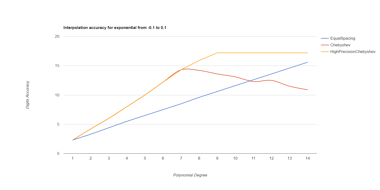
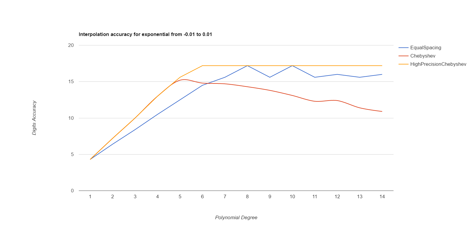
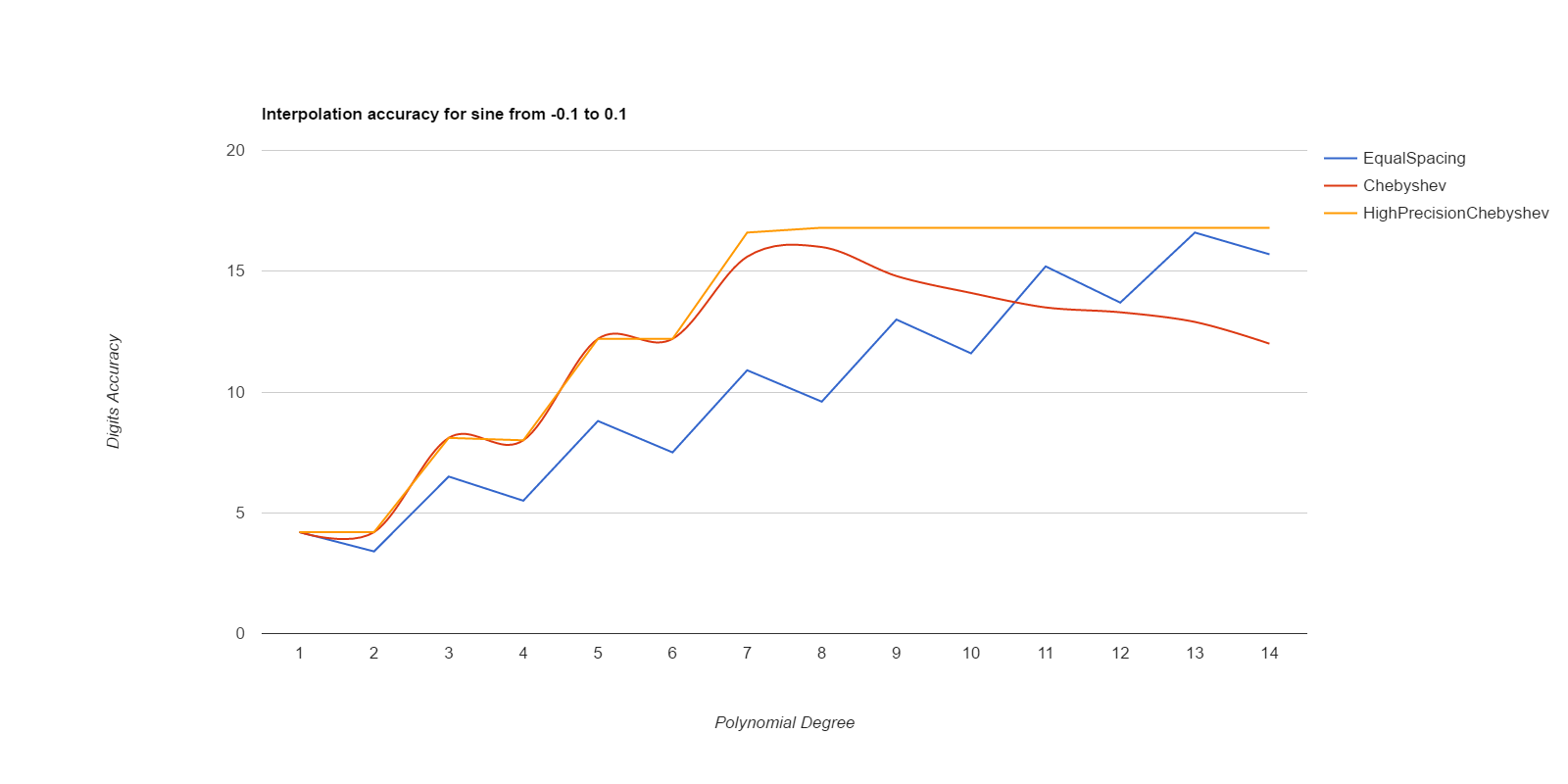
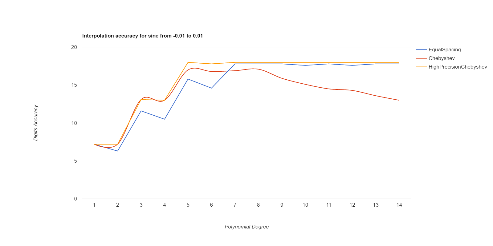
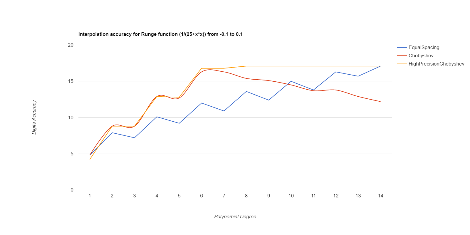
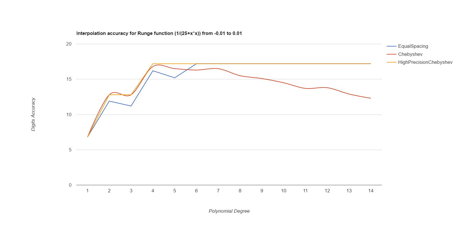
There, I measured it below (base.h, chebyshev.cpp). Equal spacing gives about the same accuracy as Chebyshev points if the equally spaced points use intervals 1/3 to 1/2 the size of the Chebyshev intervals. Here are deltas between interpolated values and ideal values, for various functions. The functions are exp(), sin(), and Runge(), where Runge is 1.0/(25.0+x*x), all over the intervals [-0.1, 0.1] and [-0.01, 0.01]. Smaller intervals converge with lower degrees, but the relative merits of the methods are the same either way. Larger intervals usually never got sufficient accuracy.

Chebyshev support are awful unless you precompute them with high precision arithmetic

EqualSpacing with even numbers of points interpolates between the middle two points, while Chebyshev uses the Chebyshev support points, which are all within the interval being interpolated over. Both use Gaussian elimination on doubles to calculate the coefficients. HighPrecisionChebyshev uses Guassian elimination with a high-precision floating point library to calculate the coefficients, then uses double arithmetic with those coefficients to do the actual interpolation. Double arithmetic is only capable of about 17 digits of accuracy.

Well, that was surprising. Chebyshev nodes did converge faster than equal spacing, but they never reached maximum accuracy, and their accuracy decays significantly starting at about 7th degree polynonmials. Meanwhile EqualSpacing eventually reaches about maximum accuracy and stays there. The inaccuracy for Chebyshev nodes seems to be due to the close spacing of the support nodes and noise in the double arithmetic doing the Gaussian elimination to find the coefficients. If higher precision arithmetic is used on Chebyshev support nodes to derive the coefficients, but the coefficients are used as doubles, that gets the fast convergence of Chebyshev nodes and retains high accuracy. When doubles are used to derive the coefficients for Chebyshev, the higher order coefficients never become small enough to be negligible, but they do come out as negligible when more accurate arithmetic is used. Using high precision to calculate the coefficients helped EqualSpacing as well, but not as much because it was already doing pretty well when using double arithmetic to calculate the coefficients.

Moral of the story: only use Chebyshev nodes if you're able to compute the coefficients with a higher precision arithmetic than you're going to be using those coefficients for. Like, use mpfr to precompute the coefficients, then use the coefficients as doubles to do the actual interpolations.

If the nth coefficient plus its 0th coefficient is the same as the 0th coefficient due to rounding of double numbers, and all further coefficients are even smaller, then there is no point in using more than coefficients 0 through n-1. It is curious that accuracy keeps improving for EqualSpacing when the higher coefficients of the polynomial are too small to possibly affect the result. I think this means the higher degree polynomials are using better coefficients for the lower degrees. Let me check that ... yes, you can get their accuracy just by using those improved coefficients for the lower degrees, and ignoring the higher degrees that cannot possibly affect the result. You can tell a coefficient is insignificant if c[0]+c[n] = c[0] in double arithmetic.

Generating an approximation of an integral of a function

Computing integrals is easy if you already have good polynomial interpolation: find the interpolation polynomials for each interval, then integrate the polynomial. This turns term cx^n-1 into (c/n)xⁿ, so if you have an initial polynomial where the nth term and beyond is negligible due to the small coefficients, then the nth term and beyond of the integral will be even more negligible.

I have everything coded well enough now to generate an accurate interpolation of the integral of a function. The coefficients are generated using Chebyshev polynomials and high precision arithmetic, but doubles are used to actually evaluate the interpolation. For example with g++ and these files

• bigfloat.h
• bigfloat.cpp
• biglagrange.h
• biglagrange.cpp
• writeinterpolate.cpp

Rings attracting points can be reduced to 1-dimensional functions

The motive for all this was a simulation that needed to measure the gravitational force of a ring on a point. That's a two-dimensional function. However, it can be expressed in closed form given function F() and G(), which are each one-dimensional. WolframAlpha pointed that out. I tried to confirm it, and found F(y) = integral of x = 0..2π of (1-ycos(x))^-3/2 and G(y) = integral of x = 0..2π of (1-cos(x))*(1-ycos(x))^-3/2 worked, but those weren't the two functions WolframAlpha was using. All the functions have a very steep pole at y=1, which I can work around by actually interpolating f(z) and g(z), where z = log(1/(1-y)) and F(y) and G(y) are as defined above. Reducing it from a 2-dimension interpolation to a combination of two 1-dimensional interpolations this way makes it a lot faster (two interpolations rather than n interpolations in x followed by an interpolation in y), and also uses way less space (kilobytes rather than megabytes to store the coefficients). It makes it small enough to ship in a javascript app.

Adaptive interpolation

It turns out that (1-cos(x))*(1-ycos(x))^-3/2 is a bathtub-shaped function, which is 0 at 0 and 2pi, smooth and low in the middle, but with peaks at either end. And as y tends towards 1, the peaks get sharper and higher. Adequately interpolating the peaks requires small stepsizes, but small stepsizes are a waste of time in the middle. As y tends towards 1, you get either inaccurate results or many-day running times or both.

The cure for this is adaptive stepsizes. We already have a criteria for when the stepsize is small enough: c_n < c₀*10e-17 where the interpolation will only use terms 0..n-1. Also the stepsize is too small (using it wastes time) if c_n-1 < c₀*10e-17. It may be that the function has naturally small c₀ or c_n, so check the top 3 terms against the bottom 3 terms instead of just comparing two terms. So you make a guess at the stepsize, see how the constants come out, then if needed double the stepsize or cut it in half and repeat. Adaptive stepsizes don't interfere with taking integrals.

Adaptive interpolation can make the interpolation function slower, because you need a series of comparisons to figure out which piece will interpolate a given point, rather than just knowing that the piece will be nPieces*(point-start)/(finish-start). On the other hand, adjusting the distribution of points so that a uniform piece size can be used (like my z = 1/(1-log(y))) is also expensive.

Implementation

Here's an implementation of all this: threehalf.cpp. point.h. ringforce.cpp. testforce.cpp. Compile it as "g++ -O3 bigfloat.cpp biglagrange.cpp threehalf.cpp -o threehalf", and running it "threehalf > th1c.cpp" will produce th1c.cpp which is an implemention of Th1c(m) = the integral of x from 1..2π of (1/(2π))*(1-cos(x))*(1-mcos(x))^-3/2. There's a line you can comment out in threehalf.cpp, then "threehalf > th1.cpp" will instead produce th1.cpp implementing Th1(m) = the integral of x from 1..2π of (1/(2π))*((1-mcos(x))^-3/2. That lets you calculate the attraction of a point to a ring in space by combining those functions in simple ways. th1.cpp is 1788 lines and th1c.cpp is 1350 lines, so these aren't particularly memory-intensive.

And here it is, integrated into a function RingAttraction() giving the force of attraction of any ring on any point. It even works for rings of zero radius, and for points at x==0 y==0, and for points very close to the ring (assuming the ring is infinitely thin and dense). The force of attraction of a ring to itself approaches infinity as the ring grows infinitely thin and dense, but if the ring has mass 1 spread across n moons, the force approaches infinity only logarithmically with n. So the best it can do without knowing the number of moons per ring is return NaN for self-attraction. "g++ -O3 bigfloat.cpp ringforce.cpp testforce.cpp -o testforce". Actually, I hardcoded it to assume there are exactly 8192 moons when the point is inside the ring.

Ringforce.cpp, which implements RingAttraction(), does not require bigfloat.cpp, it only uses point.h and the system math.h (for logarithm, I could have interpolated that too but math.h already does it and slightly better). But testforce.cpp does use bigfloat for comparison to make sure it is producing reasonble answers. Ringforce.cpp was mostly generated by threehalf.cpp .

The force between two points is antisymmetric, that is, the force of x on y is exactly the negative of the force of y on x. But I was surprised to find that the force of a ring x on a point in ring y is not antisymmetric to the force of ring y on a point in x. Consider a point at (0,0,0) (which is a ring of radius 0) and a ring of radius 1. The ring exerts zero force on the point. But the point exerts a force on any point in the ring, towards the point. It's just that if you sum over the whole ring the forces cancel out. The forces between points in rings along the z axis are indeed antisymmetric.