The Homfly Formula
The HOMFLY polynomial invariant for directed knots and links is a powerful tool for distinguishing knots and links. A recursive formula is used to calculate it. Applying this formula produces a binary tree of intermediate links. This paper presents an algorithm that encourages and collects duplicate intermediate links. It has a better time bound (and a better running time) for large links than algorithms which ignore duplicates. The time bound is O((n!)(2n)(c3)), where and c is the number of crossings in the link. n is the cross section of the link. Simple weaves are used to represent intermediate links. The basic idea behind the new algorithm is dynamic programming, but many tools and observations are needed to make this idea feasible. There is code for this algorithm, and sample inputs, online.
Knot theory is the study of knots [ 5. ]. Knots, as in sailors and shoelaces. Specifically, knot theory asks when two knots are the same. A string, intuitively, looks like a rubber band, or a piece of yarn with the two ends connected. More precisely, a string is defined to be a closed one-dimensional curve embedded in threespace. A link is any collection of nonintersecting strings. Knot theory defines a knot to be a link with only one string. A directed link is a link with a direction specified on each string (note the arrows in most of the figures in this paper). To keep strings from having an infinite number of kinks, knot theory also requires that it must be possible to approximate the arrangement of the strings with a finite number of line segments, as is done in all the diagrams in this paper.
Two links are considered equivalent, or the same, when one link can be manipulated to have the same shape as the other without breaking the strings or allowing the strings to pass through one another. (Manipulating strings really means smoothly deforming the threespace that the strings are embedded in; picture moving the air around the yarn.) The unknot is a single piece of string with no crossings, or any knot equivalent to it. An unlink is a set of nonoverlapping unknots.
A link diagram is a planar directed graph with four arcs per node, plus an extra bit per node to mark the overpass. Link diagrams look like shadows cast by a link on a plane. The nodes of the diagram are where one string segment crosses over another. The arcs in the diagram represent string segments and are directed according to the direction of the string they represent. If two links have the same link diagram, then they are equivalent.
The Three Reidemeister Moves
 \...........    \.....    \.../    \....../    \......./    \......./
 : \   --   :    : \  :    : \ :    : \  / :   -----------   : \   / :
 :   \    \ : => :  ) :    :( ): => :  )(  :    :   \   : => :   \   :
 : /   -- ' :    : /  :    : / :    : /  \ :    : /   \ :   -----------
 /..........:    /....:    /...\    /......\    /.......\    /.......\
           Type I              Type II                Type III
There are three Reidemeister moves, as shown above. A fundamental result relating the manipulation of links in threespace to the manipulation of link diagrams is that there are only three Reidemeister moves, and any manipulation of a link can be modeled as applying a sequence of these moves to a diagram of that link. A type I move undoes a loop (or makes a new loop). A type II move separates two overlapping string segments, or overlaps two separate string segments. A type III move pushes a string segment over two other crossing string segments.
Given two directed links, are they the same? If they are the same, what is a sequence of Reidemeister moves to transform a diagram of one link into a diagram of the other? No algorithm is known that is guaranteed to answer either of these questions in a finite amount of time given an arbitrary pair of links. (Since this paper was written, an algorithm that claims to do this has been found. I have not heard if this algorithm has been confirmed.) Instead of answering these questions directly, knot theory has produced a number of link invariants. If two links have the same value for an invariant, they might be the same, but if they have different values, they are definitely not equivalent links. For example, the number of strings in a link is a link invariant. The HOMFLY polynomial is a powerful invariant on directed links; it can even distinguish most links from their mirror images [ 5. ]. Computing the HOMFLY polynomial is believed to be #P-hard [ 3. ] [ 8. ].
Consider a connected region R from some directed link diagram. A weave is the arrangement of string segments in R. A weave boundary is the border of R. The three Reidemeister moves could be viewed as replacing one weave with another in a link diagram.
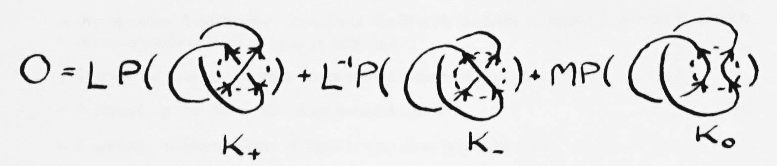
The HOMFLY knot polynomial is a polynomial with variables M and L. The HOMFLY formula relates three links which differ by weaves containing a single crossing. The first link, K+, has a right-handed crossing for this weave. The next, K-, has a left-handed crossing. The third, K0, has no crossing. There is only one way to accomplish this which preserves the directions of the strings at the weave boundary. Notice that these three knots are not equivalent; the strings generally must be broken and rejoined to transform one into another.
Link diagrams differing by an arbitrary sequence of Reidemeister moves always have the same HOMFLY polynomial. This implies that equivalent links always have the same HOMFLY polynomial, although nonequivalent links also occasionally have the same HOMFLY polynomial [ 5. ].
It can be shown that an unlink of n strings has the polynomial (M-1(-L-L-1))n-1 [ 5. ]. Another apparent property (which the author has not been able to prove or cite) is that every link's HOMFLY polynomial evaluates to some power of -2 when M and L are assigned the value 1.
How is this formula used to find the polynomial of an arbitrary link? First a crossing x in the link is chosen (assume x is a right-handed crossing). The link is plugged into K+ or K- (K+ in this case because x is right-handed). The other two links are obtained by replacing x. K- replaces x with a left-handed crossing, and K0 replaces x with no crossing at all. These new links are intermediate links. The K0 link is called the break. The other link is called the switch. The tag of an intermediate link is the polynomial that the formula has associated with it (some polynomial of Ls and Ms).
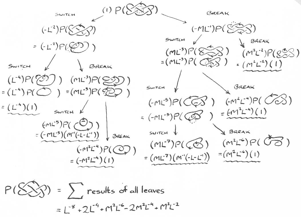
This approach will be called the binary tree approach. The leaves of the tree are all unlinks. Type I and II Reidemeister moves are applied to each intermediate link to simplify things as much as possible. There are a number of strategies for deciding which crossing to apply the formula to next. The running time of this approach is O((2c/k)(c2)), where c is the number of crossings in the link and k is some constant. k depends on the strategy used to choose crossings, and is typically around 2 [ 1. ]. The c2 comes from adding the result of a leaf to the running total polynomial. One strategy that works for choosing crossings is to apply the HOMFLY formula to the crossing that will extend the longest chain of overpasses [ 4. ].
At any point during calculation, the binary tree approach stores one copy of each link on the path from the root down to the current leaf. It does not use much memory. Every time the HOMFLY formula is applied, two entirely new copies of the link must be created and examined. Every intermediate link is treated as an isolated problem. That makes the algorithm easy to parallelize. Each time a leaf is found, its tag is multiplied by its unlink's polynomial, and the result is added to the running total. The final total is the polynomial for the original link.
Whenever intermediate links are identical, they will produce identical subtrees. Suppose we detect when intermediate links are identical, sum their tags, and only compute their subtree once. This should greatly reduce the number of intermediate links which must be examined. It may, however, be difficult to tell when intermediate links are identical. A huge number of intermediate links will need to be stored at the same time.
To make the dynamic programming approach work, the following problem must be solved. We need to find a special class of intermediate links with the following properties:
The following sections describe such a class of intermediate links. To describe the class, we must first define simple weaves and solved regions.
Consider a connected region R from some link diagram. A weave is the arrangement of the string segments in R. A weave boundary is the border of R. A boundary crossing is where a string segment crosses the weave boundary. A boundary crossing is an input if the string segment is directed into the weave. It is an output if the string segment is leaving the weave. A weave has n strings if it has n inputs and n outputs (and no loose strings in the middle). Note that every weave has an equal number of inputs and outputs. Two weaves are considered equivalent, or the same, if the string segments of one can be rearranged (using only Reidemeister moves) to produce the other. The arrangement of the boundary crossings must remain fixed.
Simple weaves are the class of weaves that have as few crossings as possible. The strings can go straight from their inputs to their outputs without getting involved in any tangles. Their boundary crossings are labeled counterclockwise, 0 through 2n-1. When strings cross, the lower labeled input must be the overpass. Any weave equivalent to a simple weave is also a simple weave.
If a simple weave is placed in standard form, the handedness and arrangement of all its crossings can be determined from just its mapping of inputs to outputs. When there is a choice about the ordering of crossings, standard form makes the string with the lower boundary crossing come first. Given a weave boundary with n inputs, for every mapping of inputs to outputs there is exactly one simple weave in standard form. Since there are n! mappings of inputs to outputs, there are exactly n! possible simple weaves with a given boundary. In fact, if you knew the boundary, you could represent a simple weave by an integer in 1..(n!).
How to arrange a simple weave in standard
form.
                ......................................
                :              +-------------------< (label 12)
                :     +--------------------------> (label 11)
                :     |        |        +-----> (label 10)
                :  +-----------------------> (label 9)
                :  |  |        |        ^ (label 8)
                :  |  |     +--------> (label 7)
                :  |  |  +--|-----< (label 6)
                :  |  |  |  |  v (label 5)
                :  |  |  |  ^ (label 4)
                :  |  |  v (label 3)
                :  |  ^ (label 2)
                :  ^ (label 1)
                :
Have all the strings form right angles as shown.
At any crossing, the string with the lowest input is the overpass.
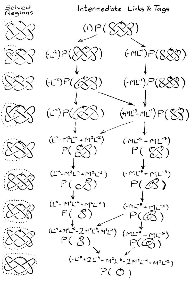
The dynamic programming approach uses a solved region to compute the polynomial. The solved region is a connected region of the original link that starts out with just one input and output. It grows by engulfing crossings one at a time until the entire link has been consumed. At any point in the computation, some of the original link will be in the solved region, with the rest in the unsolved region.
The boundary of the solved region divides the link into two parts: the solved region and the unsolved region. Reidemeister moves and the HOMFLY formula are only applied inside the solved region. Reidemeister moves that touch the unsolved region will not be allowed, even if such a move would obviously simplify the intermediate link. What is gained by this rule? All intermediate links with a given solved region have the same solved region boundary and the same unsolved region. They only differ inside the solved region.
Inside the solved region, Reidemeister moves and the HOMFLY formula can be applied until only simple weaves in standard form remain. All intermediate links have a simple weave in standard form in the solved region. Given the shared unsolved region (which includes the solved region boundary), intermediate links can be specified by just the simple weave in their solved region.
If two intermediate links have the same simple weave in the solved region, then the links are the same. Their tags can be summed, and the rest of the program can act as if they had been a single link. Given a solved region boundary with n inputs, there are n! possible simple weaves in standard form, so there will be at most n! distinct intermediate links. How can equivalent intermediate links be detected? Use their mapping of inputs to outputs to find their integer in 1..n!. If the links have the same integer, then the links are the same. The tags can even be stored in an array of 1..n!. Given the original link and the current position of the solved region boundary, the structure of each intermediate link can be deduced from a single integer in 1..n!.
This is the class of intermediate links we want: unsolved regions joined to simple weaves.
When the solved region grows by engulfing a crossing, then the intermediate links no longer have simple weaves in the solved region. Some adjacent boundary crossings changed. For each old intermediate link, Reidemeister moves and the HOMFLY formula must be applied until only simple weaves remain in the solved region.
Once everything has been reduced to simple weaves, the integers in 1..n! for the new intermediate links can be computed and their tags can be added in the new array of intermediate links. Another crossing will have been devoured.
Adding a new crossing usually switches the order of two adjacent boundary crossings. About 70% of these cases involve zero or one applications of the HOMFLY formula. The ugly cases are when one boundary crossing was an input and the other was an output, or when both were inputs (or outputs) but one was labeled 2n-1 and the other was labeled 0.
Sometimes the new crossing adds a new string to the solved region. The new solved region will have one more input than the old one did. Adding this type of crossing can always be done with zero or one applications of the HOMFLY formula.
When the new crossing connects two strings that were previously unconnected, n decreases by one but the resulting weave tends to be quite ugly.
The ugly weave has a mapping of inputs to outputs, and that mapping has a simple weave in standard form. Bad crossings are crossings in the ugly weave that differ from the corresponding simple weave in standard form. Due to the way the boundary was manipulated, all the bad crossings will be in a single string. That string was previously connected to an input with a very different label. That is where the bad crossings came from.
How is this ugly weave converted into a set of simple weaves? First the string with all the bad crossings must be found. (It is either the lowest labeled or highest labeled string that has bad crossings. It is the only string with more than one bad crossing.) Starting at the input, find the first crossing in it that is bad. Apply the HOMFLY formula at that crossing, then do any helpful Reidemeister moves. This heuristic will produce a binary tree with simple weaves at the leaves. This tree will have no more than 2n nodes. There will only be that one string not in standard form, and it will never cross itself more than twice, so the bad string will never get knotted.
When a loop gets isolated inside a weave, multiply the tag of the weave by M-1(-L-L-1) and throw away the loop.
Notice that simple weaves never have more than n2 crossings, and that explicit models of weaves are used solely to find a set of new simple weaves. Once the new simple weaves are found, the model can be thrown away. Allocating memory for models from the stack (rather than from the heap with malloc()) sped up the original implementation of the dynamic programming approach by a factor of 10.
When the current solved region has n inputs, there are at most n! intermediate links. All n! tags must be stored in memory. The most important parameter in the dynamic programming approach is n, the same way the number of crossings c determined the performance of the binary tree approach. Minimizing the maximum value of n is vital.
How big can n be? It depends on the order in which crossings enter the solved region. The Lipton-Tarjan Planar Graph Separator Theorem [ 6. ] can be used to show that n is O(sqrt(c)), where c is the number of crossings.
The dynamic programming approach is not divide-and-conquer the way most applications of the separator theorem are. Instead, crossings are added to the solved region one at a time. The algorithm depends on quickly accommodating these small changes. To choose an ordering of crossings using the separator theorem, find a separator. All the crossings on one side must be added to the solved region first, then all the crossings in the separator, then all the remaining crossings. In what order should the crossings in the first region be added? Well, this itself is a planar graph, so recurse.
A divide-and-conquer method would end up joining two solved regions, each with n! weaves. This would require n!2 operations, one for each pair of weaves. When n=8, n!=40320 and n!2 = 1625702400. Divide-and-conquer may be a bad approach for this problem.
How big can n be? It can be shown that, in the worst case, all crossings in the separator will be one-connected to the solved region. If all the recursive levels of separators were on the weave boundary, and every level of recursion has 2/3 of the crossings of the level above it (which would be the worst case using the Lipton-Tarjan theorem), then
Although this result is theoretically significant, it is useless in practice. Values of n greater than eight tend to overflow the memory of a Sun3 workstation.
The actual worst cases for n seem to be the links with n totally overlapping circles, which have n(n-1) crossings. This has not been proven in general, but it is true for n = 1,2,3,4. These links require n strings in their largest solved region boundaries. Assuming these are indeed the worst case, we can say that n <= ceil(c1/2). For most links the minimum maximum n is around (c1/2)/2.
So what is a good algorithm for deciding when to add crossings to the solved region? Finding the optimal ordering is the minimum cut linear arrangement problem, known to be NP-complete [ 2. ]. We must resort to heuristics. A greedy method happens to work well. It starts with an arbitrary crossing. At all times, some crossings are in the solved region and some aren't. Always choose the crossing that will increase the size of the solved region as little as possible. This can be done by adding the crossing which is most connected to the current solved region. If the crossing is connected to the current solved region by three strings, including it decreases n by 1. If it is connected by 2, n stays the same, and if it is connected by 1 then n increases by 1. The greedy method decreases n as soon as it can and puts off increasing n for as long as is possible.
A problem with the greedy algorithm is that it is local, and it makes many arbitrary choices. There are usually many two-connected crossings to choose from. The greedy method is good at delaying increasing n, but it is not good at decreasing n as soon as possible.
An incremental improvement is the backwards-forwards algorithm. The main idea behind the backwards-forwards algorithm is that any order and its reverse order work equally well because their solved regions have the same weave boundaries.
The backwards-forwards algorithm starts with the greedy method. It then reverses the ordering and applies the greedy method again. That's it. What is gained? When arbitrary choices are made, the first qualified crossing seen is the one that is chosen. In the first run of the greedy method, which crossing is seen first is arbitrary. But in the second run, the first crossing seen is the last qualified crossing chosen by the previous run of the greedy method. The first run is telling the second run things about crossings to come, crossings the second run hasn't seen yet. This helps the second run get to crossings that will help it decrease n sooner.
The backwards-forwards algorithm almost always minimizes n, and often minimizes the number of crossings that must be added while n is at its maximum. It may be useful for other vertex ordering problems as well.
m: the number of inputs into the old solved region
n: the number of inputs into the new solved region
c: the number of crossings in the original link
old[m!]: array of tags of old intermediate links
new[n!]: array of tags for the new intermediate links

Use the backwards-forwards algorithm to choose the order in which to
  add crossings to the solved region.  Number them 1..c.
Build an initial solved region
    Its boundary has one string, so m := 1;
    It is next to the first crossing to be added;
    It contains one simple weave;
    The tag of the weave is 1, that is, old[i] := 1;
For each crossing 1..c,
    Describe how adding that crossing to the solved region changes its boundary
    Compute n
    For i = 1..n!,
        new[i] = 0;
    For i= 1..m!, if old[i] has a nonzero tag,
        Use i to reconstruct the simple weave in standard form;
        Add the new crossing to the simple weave;
        Recursively apply the formula and Reidemeister moves
          until you only have simple weaves left;
            For each new simple weave
                Compute the integer j for its mapping of inputs to outputs;
                Add its tag to new[j];
    old := new;
    m := n;
We are left with the final solved region
    Its boundary has one input, so m := 1;
    It is next to the last crossing added;
    It contains one simple weave;
    This final intermediate link is the unknot and the polynomial of
      the unknot is 1;
    The link's tag, old[1], is the polynomial for the whole original link.
Return old[1].
These are some things that still need to be proven about the dynamic programming approach.
These are some possible extensions and uses of this algorithm.
The dynamic programming approach has a time bound of O(n!(2n)(c3), where n <= 8.85c1/2. This bound on n was determined by the planar separator theorem. The actual value of n found by the forwards-backwards algorithm is usually around (c1/2)/2, and is probably always at most ceil(c1/2). The n! is for the maximum number of intermediate links at any given time. The 2n is the maximum number of steps needed to reduce an old intermediate link to a set of new intermediate links. The c2 is the maximum size of a tag, and the third c comes from the fact that this whole process is done for every crossing in the link. The dynamic programming approach also takes O((n!)(c2)) space, because all the tags for all the intermediate links with a given solved region must be stored simultaneously. Space tends to be the Achilles' heel of the dynamic programming approach.
Experiments have shown this approach to be faster than the binary tree approach for most links with over 13 crossings. One random 56 crossing link (n = 5) took 8 seconds to solve on a Sun3 with the dynamic programming approach. The binary tree approach ran for 1 1/2 hours before it was killed out of boredom.
More recently, an O(2O(sqrt(c))) algorithm was found by K. Sekine and S. Tani for computing the Jones' polynomial based on the Tutte polynomial for undirected graphs [ 7. ]. This new algorithm also uses the planar separator theorem, and an elimination boundary, and dynamic programming. A comparison of the techniques here and there seems worthwhile.
Back to the Table of Contents