By
Robert J. Jenkins Jr.
Submitted in partial fullfillment of the requirements for the degree of
Masters of Science in Mathematics
Department of Mathematics
Carnegie Mellon University
Pittsburgh, Pennsylvania
June, 1989
This paper presents an algorithm for computing the Homfly polynomial invariant for oriented links of c crossings in O(n!) space and O((c)(n!)(2n-1)) time, where n is at most ⌈√c⌉. A few properties of the Homfly polynomial, of weaves, and of links in general are explored as well.
The topic of this paper is a new algorithm for computing the Homfly polynomial. This is not the topic I originally intended to write about. The original title was A Survey of Knot Theory, and the paper was to list and prove the major known results about links. I did not intend to present any new material.
As it turns out, the latter half of this paper is all new material. I was unable to locate many of the proofs I had counted on for writing the original paper. The proofs that I was able to create on my own were long, unenlightening, and complicated. A month before the thesis was due I decided to give up on my original intentions and develop this algorithm instead, which I had stumbled upon in the meantime. I finished this paper and an implementation of the algorithm a month after the paper was due.
I wish to thank Daniel Sleator for proposing this topic and for being my advisor throughout the whole ordeal. I thank Peter Freyd and Richard Statman, my committee members, for the useful advice they have given me. I thank Niel Calkin for taking part in the defense. I thank David Owen for his support over the last two semesters, and Walter Noll, Bill Williams, and Juan Schaeffer for training me how to think like a mathematician. I thank my parents for encouraging me to do my best. Finally, I thank Freyd, Lickorish, Kauffman, Fox, Birman, Conway, Reidemeister, and all the others who have contributed to the rich literature of Knot Theory, without which none of this would be possible. Of course, I take complete credit for all my mistakes.
Knot theory is the mathematical study of knots — you know, boy scouts and shoelaces. Specifically, knot theory is concerned with determining when two links are actually the same. Knot theory does not consider how useful a link is, how likely a link is to slip, how much it weakens the rope it is tied in, or even what it looks like when tightened. Knot theory is only concerned with determining if two links are actually the same.
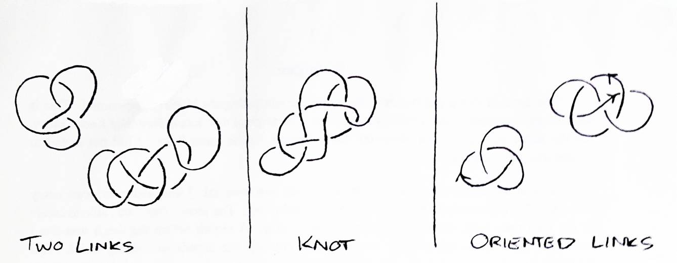
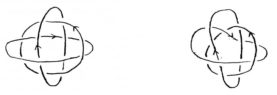
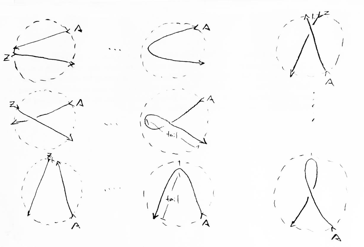
A link is the union of a set of disjoint closed curves embedded in threespace. Each curve will be referred to as a string. A link looks like a bunch of physical strings, perhaps tangled and knotted, where every string has its two ends connected. A knot is a link with only one string. An oriented link is a link which has a direction specified on every string (see Figure 1). In order to assure that the kinks and tangles of the link aren't of infinite complexity, it is assumed that all the strings in every link are differentiable. It would do equally well to assume each string is actually a union of a finite number of line segments placed end to end [2].
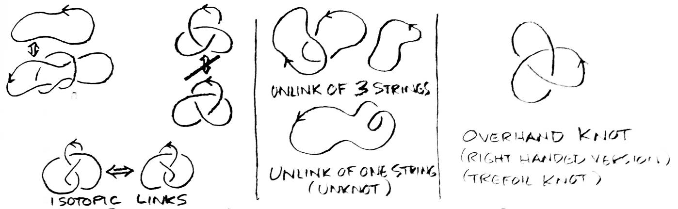
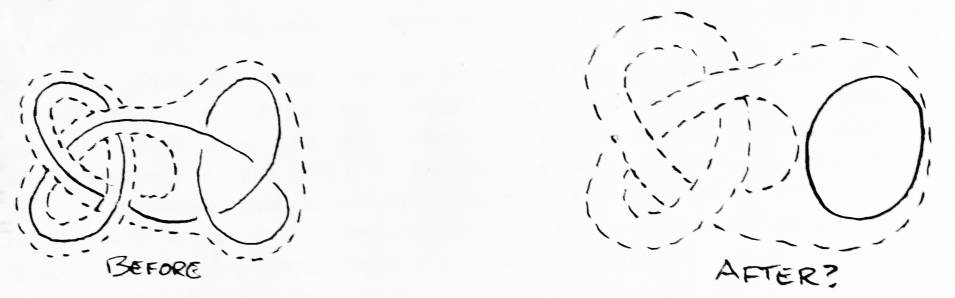
Two links are considered the same (or isotopic) if it is possible to manipulate one to look like the other without breaking the strings. Such a manipulation, taking a link from rest to some final state, is called an ambient isotopy. Actually, an ambient isotopy requires manipulating all of threespace (picture the air being moved as you manipulate the link), but it can be proved that if you can just move the link, you can move all of threespace as well. An unknot is a knot which is isotopic to a circle. An unlink of n strings is a link isotopic to n isolated circles. Even though the overhand knot has only one string, it is not isotopic to a circle, so it is not an unknot (see Figure 2).
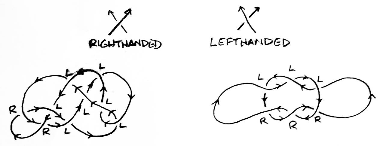
Almost always, links are dealt with through their regular projections onto a plane. A regular projection is best thought of as a drawing of a link with a finite number of crossings. Every string must have a direction, every crossing must have only two string segments involved (with the overpass distinguishable from the underpass), and the string segments at each crossing must actually cross, not just overlap. Every crossing is either right or left handed. Point the thumb of your right hand in the direction of the overpassing string segment and curl your fingers under. If the underpass goes in the direction of your fingers, it is a right hand crossing. Otherwise, it is left handed (see Figure 3).
A regular projection can be represented in a computer by an array of crossings and a cyclic linked list for each string. The linked list would have one node for each time the string passes over a crossing, and the value of that node would be the name of that crossing. Each crossing in the array of crossings would be a triple (overpass node, underpass node, handedness). This representation is more like a four-regular directed graph with added structure than it is like a jumble of strings. The exact positions of the strings is ignored; all that matters is how the crossigns are arranged. If two links have the same regular projection, they are isotopic. Although this may seem obvious, the proof of it is very ugly (and won't be given here).
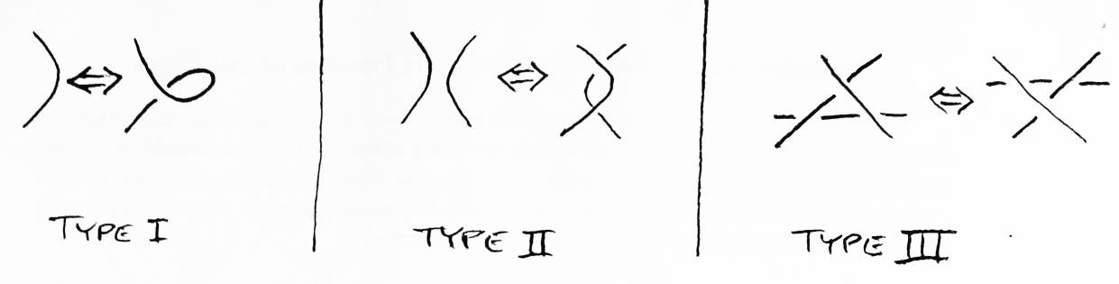
A fundamental result in knot theory is the sufficiency of Reidemeister moves [1]. Reidemeister moves are three types of changes that can be made to the arrangement of crossings in a regular projection such that the new regular projection will be isotopic to the original one (see Figure 4). There is a theorem that two regular projections represent isotopic links if and and only if there is a sequence of Reidemeister moves that change one projection to the other (see Figure 5). Unfortunately, given two regular projections, there is no general algorithm for generating such a sequence of Reidemeister moves, or even determining if such a sequence exists.
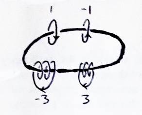
An invariant on an oriented link is a property or value that is associated with a link and does not change no matter how the link is manipulated. The number of strings in a link is an invariant. The minimum number of crossings the link's regular projection may have is an invariant. If two links have different values for a given invariant, then those links are certainly not isotopic. If the links have the same value, they might be isotopic, but then again, they might not. The values of invariants are like a name — if two given people are named Bob and Tom, they are different people. If they are both named Bob, they might still be different people (see Figure 6). The more unlikely it is for two different links to have the same value for a given invariant, the stronger that invariant is considered to be. The history of knot theory has been a search for stronger and stronger invariants, and for easier ways to compute those invariants.
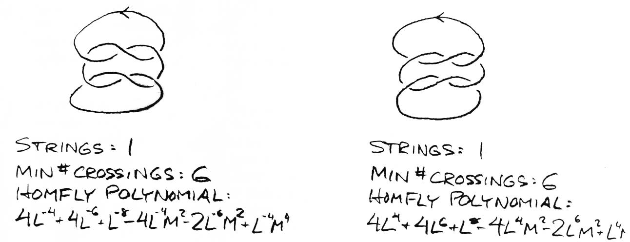
The Homfly polynomial and the related recursive polynomials [8][9], which are generalizations of a polynomial discovered by Vaughan Jones in 1984, are exteremely powerful invariants on links. Their computation usually involves traversing binary or trinary trees with a depth of the number of crossings in a regular projection of a given link. This exponential time bound limits their use mostly to links with regular projections of thirty crossings or less. The subject of this paper is an algorithm for the Homfly polynomial which does not suffer from this exponential time bound. It is still exponential, but it is roughly exponential on the square root of the number of crossings. It is capable of determining the polynomial for knots with hundreds of crossings in a reasonable amount of time.
For example, I have a link with 56 crossings I was debugging my program wth. My program computes the polynomial by looking at 1372 intermediate knots, and it runs in 8 seconds on a Sun workstation. I also tried to compute the Homfly polynomial for this knot using a program that ran on the previous method (the binary tree), but I calculated it would take two days to figure it out. After half an hour of grinding, I just killed the process. The point had been made. For all knots that both programs can solve, both programs produce the same result.
One of the earliest known invariants on knots was the knot group[2][4]. The fundamental group of a space is the group of all homotopic oriented closed loops in that space. Two loops are homotopic if you can move one to look like the other (it's like isotopic, except you're allowed to pass the loop through itself in a homotopy). The fundamental group of just threespace is trival, since every loop can be deformed to look like any other loop. The fundamental group of threespace with a circle taken out of it is equivalent to the integers (depending on how many times the loop goes through the circle, and in what direction). The knot group of a link is the fundamental group of the complement of the link in threespace. It has been proven that the unknot is the only link with a knot group isomorphic to the integers [4] (see Figure 7). It has been conjectured that there are no two distinct prime knots (ignoring reflection and reversal of orientation) which have the same knot group.
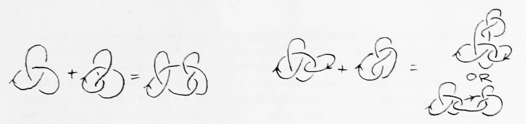
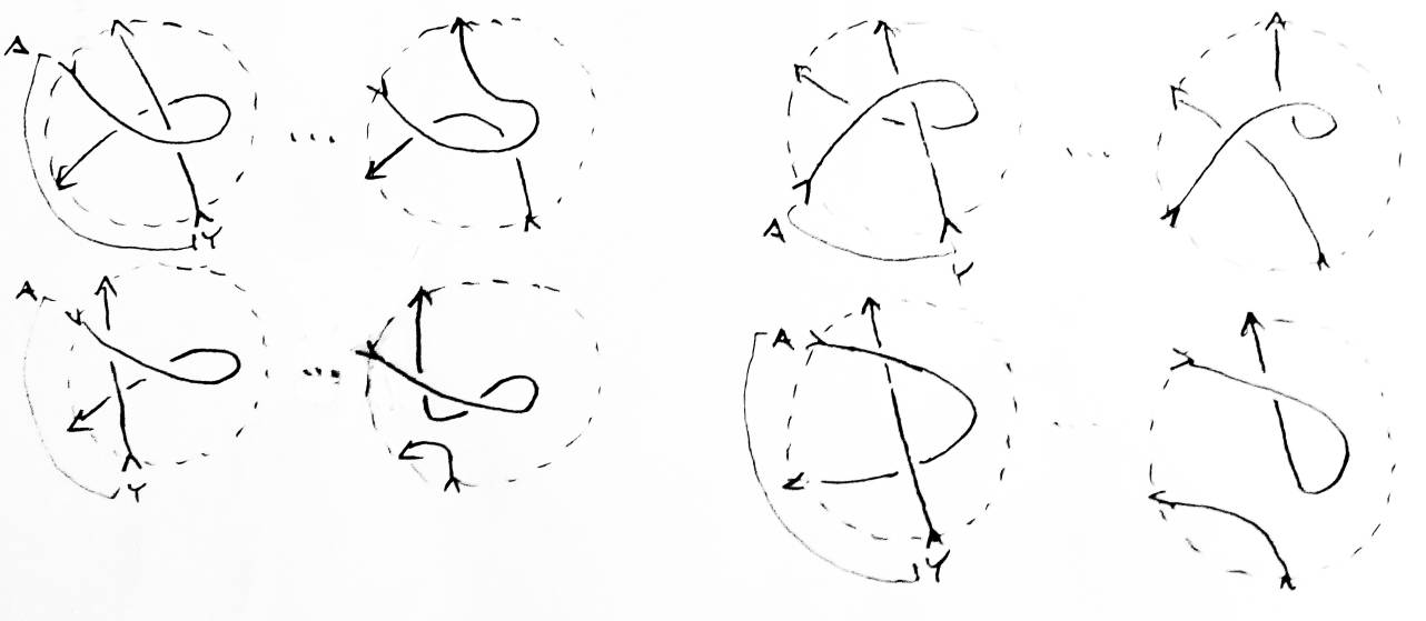
Given two oriented knots, their sum can be formed by placing the two knots side by side, breaking their strings, then connecting their strings to each other (pairing the strings so they preserve their orientation) (see Figure 8). The sum of two oriented knots is unique — shrink down one knot real small and slide it along the other's string, and you can duplicate having made the sum anywhere. A prime knot is a knot that is not the sum of two other knots Knot tables generally only list prime knots. The sum of two links is not necessarily unique — if the sum is made to different strings in a link, different links can be produced.
Prime knots cannot be canceled by other prime knots (unless both are really the unknot). To show this, picture the sum of two knots with a shell surrounding it such that the shell is actually one of the knots itself (the other being totally engulfed by the shell) (see Figure 9). Now consider an ambient isotopy that lets the two knots that form the sum cancel each other, leaving a circle. What happened to the shell? Ambient isotopies are continuous, so the string always stays in the shell. The shell is still a knot, because (by definition of prime knot) no ambient isotopy can deform a prime knot into the unknot. So the string must now be in only part of the shell. Consider a cross section of the shell after the isotopy which does not intersect the knot. Trace the isotopy backwards. Where was our cross section then? In the original state, every cross section intersected the knot. Therefore, no such ambient isotopy can exist, so prime knots cannot cancel each other out. This proof has been attributed to J. H. Conway.
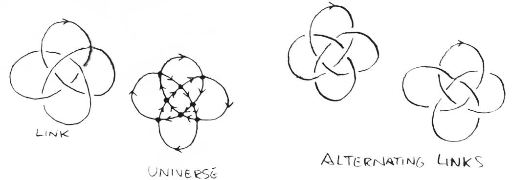
An alternating link is a link which has a regular projection such that no string has two consecutive underpasses (or overpasses). (There are an equal number of underpasses and overpasses in a link, so if there are two consecutive underpasses, there must be two consecutive overpasses.) The universe of a regular projection is the set of all regular projections which, ignoring which strings are the overpasses and underpasses at the crossings, are the same as the given regular projection [7]. A universe can be represented as 4-regular planar graph. Every universe contains two alternating links (see Figure 10). Let a universe be given. Let a line crossing the universe be given. Choose a point on the line and count how many times the halfline to the right has crossed the projection. If the count is even, then color the region that the point is in black. Otherwise color it white. This method can be used to color the plane so all the white regions are adjacent to only black ones, and vice versa. Now go around every black region clockwise, drawing overpasses to underpasses on the border. This is an alternating link for this universe. Drawing underpasses to overpasses produces the other alternating link. A recent theorem in knot theory states that any alternating regular projection (free of type I Reidemeister moves, or whole sections that can be flipped over to eliminate a crossing) has a minimum number of crossings for the link it represents [7][9].
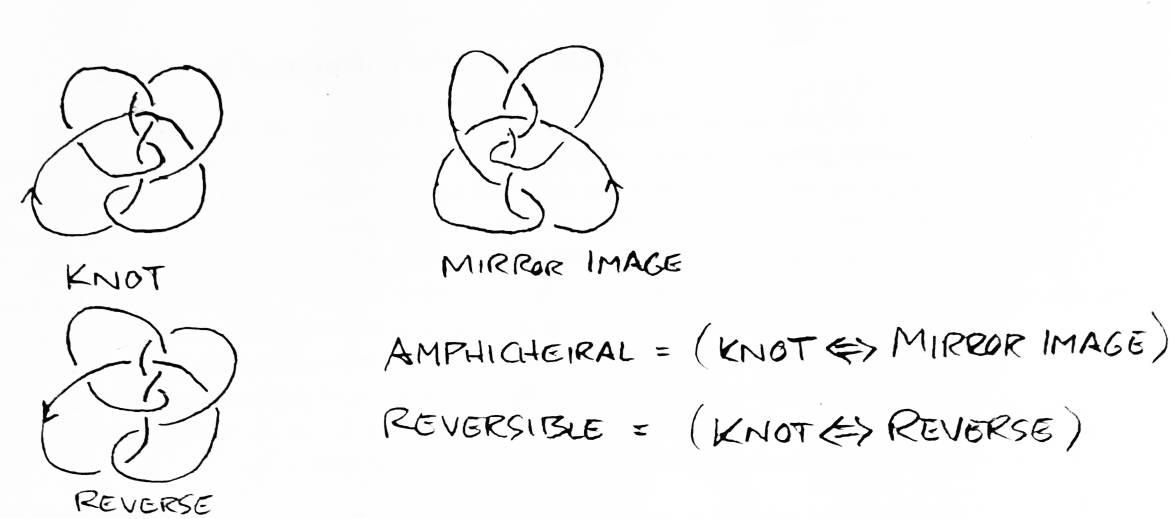
The knot group of an oriented link cannot distinguish a link from its mirror image. Links which are actually isotopic to their mirror image (the figure eight knot, for example) are called amphicheiral. Knots which are not isotopic to their mirror image are called cheiral. Some oriented knots are even irreversible, meaning that they are not isotopic to the oriented knot obtained by reversing the knot's orientation (see Figure 11). Since the orientation of a link is irrelevant to the definition of a fundamental group, it is clear that the knot group also cannot distinguish a knot from its reverse. The worst problem with the knot group, however, is the difficulty involved in comparing the knot groups of two knots. Every knot group has many presentation, and determining if two presentation represent the same gorup is almost as hard as finding a sequence of Reidemeister moves to transform one knot into the other.
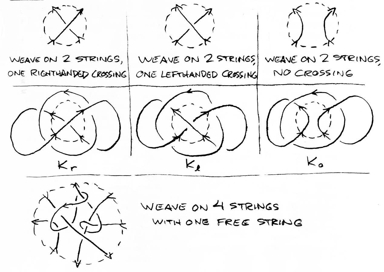
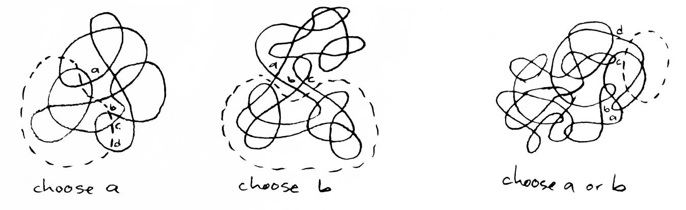
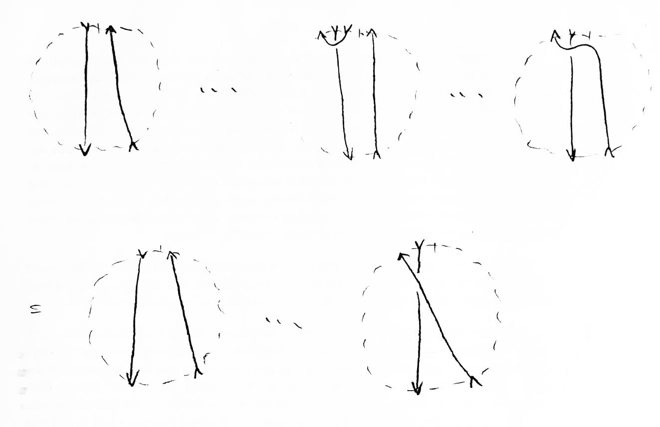
Take a regular projection. Draw a circle on it. The region of the projection within the circle will be called a weave. A "weave" is similar to the plats used in [3]. Weaves also closely resemble W. B. R. Lickorish's tangles [6], although the boundaries of weaves, unlike tangles, are fixed. A weave is said to have no free string if every string in the weave crosses the weave's boundary. A weave of n strings is a weave whose border is crossed 2n times (each string goes in and out). An input is a crossing of a weave's border by a string going into the weave. An output is a border crossing by a string leaving the weave. Given an oriented link K with a weave of 2 strings enclosing just one of its crossings, we define Kr, Kl, and K0 to be the links that are exactly like K, except with the weave replaced by a weave with a right hand crossing, a left hand crossing, and a weave with the inputs matched to the outputs so there is no crossing (respectively) (see Figure 12).
In 1926, a polynomial invariant on links was discovered by J. Alexander [2][9]. The Alexander polynomial for a given link is derived from the link's knot group. Although the Alexander polynomial is still a very strong invariant, it inherits all the knot group's weaknesses and has some more of its own. The unknot has an Alexander polynomial of 1. There are also other prime knots with an Alexander polynomial of 1. In 1960, Conway discovered a recursive method for computing the Alexander polynomial. Let K be an oriented link, and let a weave single out one its crossings. Let Δ(X) represent the Alexander polynomial for a link X. Let O be an unknot. We define Δ, the Alexander polynomial, by saying Δ(O) = 1 and
In the spring of 1984, Vaughan Jones created a polynomial invariant on oriented links which contained the Alexander polynomial as a special case. This new polynomial could distinguish all the knots the Alexander polynomial could, and more. It could distinguish many knots from their mirror images. This new polynomial could also be calculated recursively, and its formula was very similar. Again, let K be an oriented link with a weave singling out one crossing and let O be the unknot. Let V(X) be the Jones polynomial for a link X. We define V, the Jones polynomial by saying V(O) = 1 and
Later that year, Freyd, Yetter, Hoste, Lickorish, Millett, and Ocneanu independently generalized Jones' polynomial to a polynomial in two variables (or three variables, where one is determined by the other two). This generalized Jones polynomial is called the Homfly polynomial, the name of which is an anagram of the initials of everyone who discovered it [8]. This polynomial is also determined recursively. Let a link K be given, and let a weave single out one of its crossings. Let P(X) be the Homfly polynomial for the link X. We define P, the Homfly polynomial, by saying P(O) = 1 and
Proving that the Homfly polynomial is uniquely determined for a given regular projection, and that it is invariant under the Reidemeister moves, is not a pleasant thing to do. I will not present any type of proof for it here. The outlines of a number of proofs, given by the mathematicians who discovered the polynomial, appear in [8]. Also, there is a natural urge to ask just what M and L stand for in the polynomial. They don't stand for anything. The polynomial is, effectively, just a name for a link, and M and L are the letters in that name. Before presenting the new approach to calculating the Homfly polynomial, we will explore some of the properties of the polynomial and work through a couple examples of it by the old method. I found most of these properties in [9].
Again, the Homfly polynomial is defined recursively. Let P(X) be the Homfly polynomial for the oriented link X. Let K be an oriented link with a weave singling out a crossing and let O be the unknot. Then P(O) = 1, and
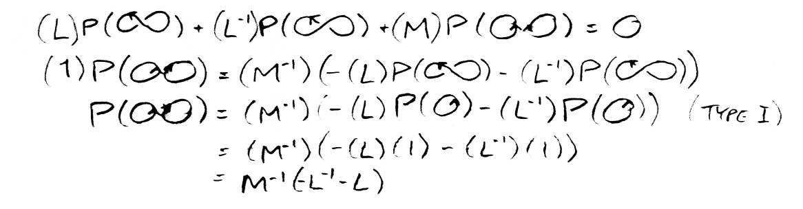
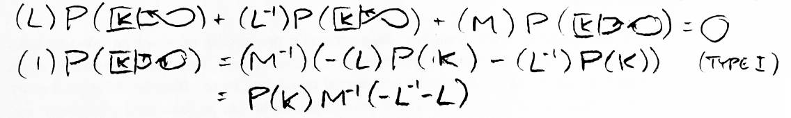
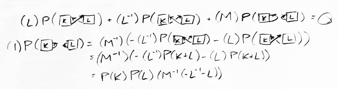
The polynomial for the unknot is 1. What is the polynomial for an unlink with two strings? That requires only one application of the main formula (see Figure 13). What is the polynomial for anything unioned with the unknot? In Figure 14 it is shown to be P(K)M-1(-L-1-L). From this we can conclude that the polynomial for an unlink of n strings is (-M-1(L-1+L))n-1.
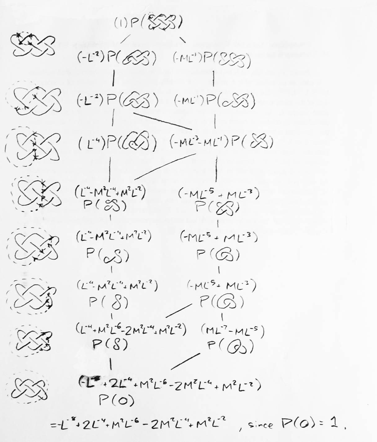
Using this knowledge, we can avoid ever having to solve for K0 in the formula again. As an example, let us look at a more complicated case (see Figure 15). Each application of the formula replaces a link (either Kr or Kl in the formula) with two other links (K0 and either Kl or Kr). A binary tree of links, which I call a formula tree, is formed this way. All the leaves of the tree are unlinks. The path of the tree ending with a given leaf associates a polynomial with that leaf (to be referred to as the path polynomial). By multiplying the path polynomials by the Homfly polynomials for these unlinks, then adding up all the resulting polynomials, we get the polynomial for the original link (the root of the tree). A child in the tree resulting form chanigng the handedness of a crossing is called a switch. A child resulting from removing the crossing altogether is called a break.
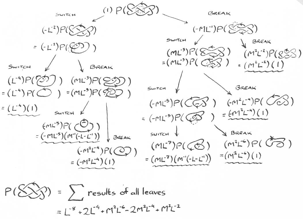
Given a link whose polynomial we wish to compute, which crossing should we apply the formula to? How do we know our binary tree will be of finite depth? There is an easy way to answer both questions. Given a link, apply the Homfly formula to the crossing which contains the underpass following the longest chain of overpasses. The link resulting from a switch will have a longer chain of overpasses. Eventually this chain of overpasses will cross under itself. All its crossings can then be removed, effectively a large Type I Reidemeister move, without changing the polynomial. The link resulting from the break will have fewer crossings than its parent. Any link with no crossings is an unlink. Hence the tree will be of finite depth. Since Reidemeister moves do not change a link's polynomial, it is advantageous to remove from each link as many crossings as possible by Reidemeister moves before reapplying the formula. The fewer crossings there are, the fewer links which have to be considered. This is the method used in the example in Figure 15.
There are a number of characteristics of links that can be seen in their polynomials. Perhaps the easiest to see, and the best selling point for the Homfly polynomial, is the way it determines chirality. Once again, a knot is cheiral if it is different from its mirror image. The only difference between a link and its mirror image is the handedness of their crossings.
Proposition: If K is a directed link and P(K) is f(M,L), then if f(M,L) is not equal to f(M,L-1), K is cheiral.
Proof: The mirror image of a link changes all righthanded crossings into lefthanded ones, and vice versa. Given a link X, the Homfly formula associates L with Xr and L-1 with Xl. The formula tree used to compute a link can just as easily be used to compute its mirror image. The only difference is that L is replaced everywhere by L-1. The Homfly polynomials for all unlinks are symmetric with respect to L and L-1. Therefore the polynomial for the mirror image of a link is exactly that of the link itself, except with L replaced everywhere with L-1. If the polynomial for a link is not symmetric with respect to L and L-1, then the link is cheiral. The converse, unfortunately, is not true (see Figure 16). ∎
Proposition: If K and L are links with polynomials P(K) and P(L), then P(K+L) = P(K)P(L).
Proof: Let two links K and L be given, and let K+L be a sum of K and L (see Figure 17). Place the boundary of a weave around K in K+L. This is a weave of one string, although it may have free strings as well. Try to compute the Homfly polynomial for K+L by the method described above, but only choose crossings inside the weave, and do not use Reideymeister moves that change anything outside the weave. The final formula tree will have, at each leaf, L and a bunch of circles. One string of L will pass through the weave, but there will be no crossings inside the weave. At each leaf, for each free circle, multiply the path polynomial by M-1(-L-1-L) and throw away the circle. This leaves, at each leaf, just L and the path polynomial. Since the sum of products is the product of sums, we may sum all the path polynomials (to get P(K)) and build the rest of the formula tree for K+L as if there were only one leaf of the current tree (with L as its link and P(K) as its path polynomial. Every path polynomial will be multiplied by P(K), so the final polynomial will be P(K)L(K). ∎
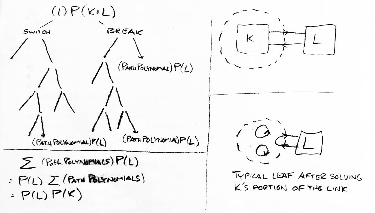
What is the Homfly polynomial for the link K∪L? Using the preceding property, this can be easily seen to be P(K)P(L)(M-1(-L-1-L)) (see Figure 18). Using this property, we can restrict our attention to links of only one component.
Proposition: A mutation or a link can be created by choosing a weave of two strings on the link, then cutting the weave out and pasting it in again so the directions of the strings hasn't been changed, but every string is attached differently (see Figure 19). If two links differ only by a mutation, then their Homfly polynomials are the same.
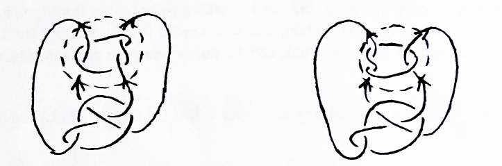
Proof: Let a directed link K be given, and specify in it a weave of two strings. Apply the formula to crossings inside the weave. Never using Reidemeister moves that affect anything outside the weave. Stop when the weaves at the leaves have as few crossings as possible. (Since paths that are all switches cannot change what inputs go to what outputs, some weaves may need to retain one crossing.) At each leaf, for each free unknot, get rid of the unknot by multiplying the path polynomial by M-1(-L-1-L). Sum all the path polynomials for leaves that now have the same weave to get weave polynomials (there are either two or three distinct weaves, depending on if the inputs are arranged to require a crossing in the weave). Each weave connects to the rest of K to from a link. In all of these new links, a mutation of the weave leaves the link unchanged (see Figure 20). The polynomial for K is the sum of the polynomials for these new links times their weave polynomials. Since the new weaves were derived from the original one without reference to the rest of K, mutating the original weave would have the same effect on the polynomial as mutating all the final weaves — no effect at all. The mutation of the original weave would produce a link with the same polynomial as K. ∎
Proposition: Let an oriented link K be given. If K has an odd number of strings, every term in P(K) will have only even exponents. If K has an even number of strings, every exponent in P(K) will be odd.
Proof: This can be proven by induction with the unlinks as the base case. The proposition holds for unlinks. Now look at a formula tree computing the polynomial for a given K, and assume the claim holds for the children of K. The switched child has the same number of strings as K, and its polynomial is multiplied by L2 or L-2, depending on whether the switch produced Kr or Kl. Hence the terms for P(K() coming from the switch will have the right type of exponents. The broken child has either one more or one less string than K (depending on whether the crossings in K involved the same string or two different strings). The broken child's Homfly polynomial will, by the induction hypothesis, have odd coefficients if K's is supposed to be even, or even if K's is supposed to be odd. This polynomial is multipled by ML or ML-1, depending on wehther the crossing in K was left handed or right handed. Hence the terms of P(K) coming from the break will have the right type of exponents. Hence the terms of K have only even or only odd exponents, depending on whether K has on odd number or even number of strings. ∎
Proposition: Let a link K be given. The lowest power of M appearing in P(K) will be M1-n, where n is the number of strings in K.
Proof: To see this, let K and the formula tree for K be given. Follow the path of all switches — it ends in an unlink with n strings. The Homfly polynomial for an unlink of n strings is M1-n(-L-1-L)n-1. The path polynomial for the path of all switches is some power of L2, so the sum of terms contributed to P(K) by the path of all switches will be L2x(M1-n(-L-1-L)n-1) for some integer x. Let another path in the formula tree for K be given such that all the terms contributed by it have M raised to the power (1-n). Since they are not the path of all switches, they involved a break somewhere in their path. Breaks multiply path polynomials by M (and either L or L-1). In order to reduce the power of M back to M1-n, the unlink at the end of the path must have more than n strings. Thus the sum of all the terms contributed by this path are a multiple of (-L-1-L)n. Consider P(K) mod (-L-1-L)n. The only remaining terms in P(K) with M1-n as their power of M will be those from the path of all switches. Hence P(K) will never be 0 for any link K, and there will be terms in P(K) with M1-n as their power of M. Furthermore, there will be no terms with lower powers of M. Multiplying by M-1 can only be done by having extra strings. Extra strings can only come from breaks. Breaks always multiply by M. Hence no term in P(K) will have a power of M lower than M1-n. Therefore, no link has a polynomial of 0, and the lowest power of M in the polynomial for a link K is M1-n, where n is the number of strings in K. ∎
(It will be assumed from this point on that all links have only one component. Those with more can have their polynomial computed using the fact that the Homfly polynomial for the disjoint union of links K and L is P(K)P(L)(M-1(-L-1-L)).)
The Homfly polynomial for a given link can be computed incrementally, using weaves. This method divides a link into a sovled region and an unsolved region, separated by a weave boundary. The solved region is represented by a set of weaves and the polynomials associated with them, and represents all the crossings in the link that have already been dealt with. The unsolved region is just the region of the original link that has yet to be dealt with. The polynomial associated by the algorithm with a given weave W is called the weave's tag, denoted TW. The solved region starts with a piece of string to the side of one crossing, then engulfs crossings one at a time until the solved region is the entire link and the unsolved region is empty (see Figure 21). Picture a line of fire slowly turning piece of paper to ash. That is how this method works.
All the weaves representing the solved region have the same boundary (the weave boundary passing through the strings that connect the solved region to the unsolved region). Applications of the formula for the Homfly polynomial can change the interior of a weave but they can't change the boundary. All weaves will have the same inputs and the same outputs, so they have to have the same number of strings. Which input connects to which output, however, will differ from weave to weave. There are n! ways to match n inputs to n outputs. Since all the links in the path of all switches in a sequence of applications of the Homfly formula always matches the inputs to the same outputs, if you have n strings in every weave, you may be required to represent the solved region by n! weaves. For this reason, it is a good idea to keep the number of strings in every weave as small as possible.
Theorem: Given a link K with c crossings, the crossings of K can be added to the solved region in such an order that the number of arcs connecting the solved region to the unsolved region is O(√c).
Proof: An arc is a segment of string connecting two crossings. Let a link K with c crossings be given. K's link universe is a 4-regular planar graph with c vertices. By the planar separator theorem of Tarjan and Lipton, the vertices of any planar graph can be partitioned into three sets A,B,C, such that no edge joins a vertex in A to a vertex in B, neither A nor B contains more than 2n/3 vertices, and C contains no more than 2(√2)(√c) vertices. C is a separator for the graph [5]. The 2√2 was later reduced by Djidjev to √6. By partitioning the link universe of K by this theorem, then by recursing on the subgraphs with vertices in A and with vertices in B, the crossings of K can be partitioned into separators and isolated crossings. The crossings in a set can be ordered in this manner: divide the set into sets A,B,C as above, put all the crossing in A first and order the points in the set A, put all the crossing in B next (any order), put all the crossings in C last and order the crossings in C. If a set has only one crossing, let it be. The original set would be all the crossings of K. By adding the crossings of K to the solved region in this order, the largest number of crossings in the unsolved region adjacent to the solved region (and vice versa) would be all the crossings on all the separators separaitng the crossings in the solved regions from those in the unsolved. This means there can be at most 3 times the number of arcs connecting the solved regions to the unsolved. This number of crossings is the limit, as n goes to infinity, of the sum for i=1 to n of (√6)sqrt((2/3)ic), or (√6)1/(1-sqrt(2/3))(√c), so there are at most (3)(√6)(1/(1-sqrt(2/3)))√c, or about 40√c, arcs connecting the solved region to the unsolved region at any time. Hence the maximum number of arcs joining the solved region to the unsolved region need not exceed O(√c). ∎
A greedy method for ordering the crossings in a link happens to work better than the method outlined above. Given the first x crossings to be added to the solved region, choose the (x+1)th by this method: always add the crossing in the unsolved region that is connect to the solved region by the most arcs. If a crossing is connected by three arcs, adding it decreases the number of strings in all the weaves by 1. If the crossing is connected by two arcs, the number of strings stays the same. If the crossing is connected by by only one arc, the number of strings in every weave increases by 1. If all prospective crossings are connected to the solved region by only one arc, choose the prospective crossing that is connected to the most other prospective crossings (see Figure 22).
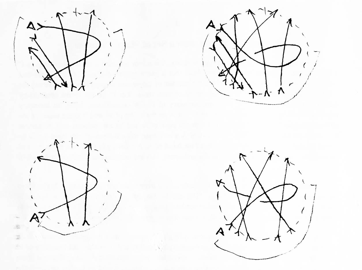
Given a link K with c crossings, I claim an ordering of the crossings can be chosen so that no weave has more than (1)(⌈√c⌉) strings. (It is difficult to find examples in which the greedy method of ordering might exceed that.) I claim that the smallest links which require weaves of n strings are links of n strings, where no string crosses itself and every string crosses every other string twice (once going in, once going out) (see Figure 23). These links have (n)(n-1) crossings. They require weaves with n strings because no string in the link can be engulfed by the solved region without touching every other string in the link first. I cannot prove either of these claims at the present time, although the claim about the smallest links requiring weaves of n strings is true for n=2,3, and 4.
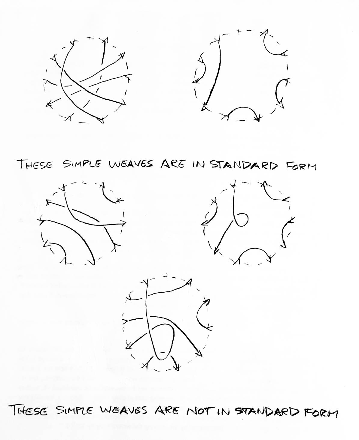
Recall that a weave was defined to be a region of a regular projection of an oriented link — draw a circle on a regular projection, and anything inside or on that circle is the weave. Weaves have strings going in (inputs) and strings going out (outputs). A weave with n inputs is said to be a weave of n strings. Weaves may contain strings which never cross the boundary at all. Such strings are said to be free strings. Hence the set of all oriented links is actually a subset of the set of all weaves (specifically, they are the weaves of no strings, where all the string in the weave are free). Weaves can be really ugly.
In order to avoid the full ugliness of weaves, we introduce the concept of a simple weave. A simple weave (see Figure 24)
Let a link L with a weave X be given. If Y is a weave with the same boundary as X, then LY is the link obtained by replacing X in L with Y. Recall that the polynomial associated with a weave W, called the tag of W, is denoted TW. Replacing the weave X with a set of simple weaves S means using Reidemeister moves and the Homfly formula to obtain a set of simple weaves S such that TXP(L) is the same as the sum of TYP(LY) for all simple weaves Y in S.
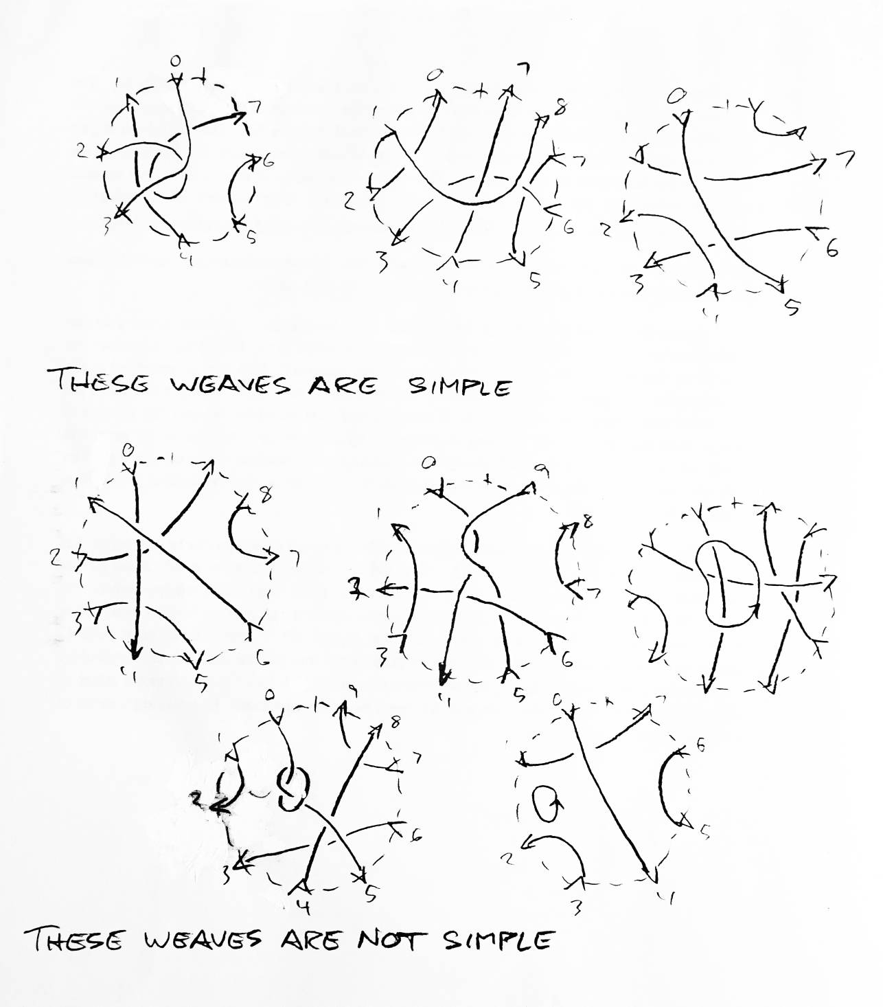
Theorem: Any weave on n strings can be replaced by a set of not more than n! simple weaves.
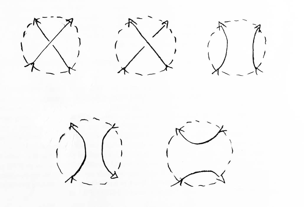
Proof: Let a weave be given. Let a strating point on its boundary be given, and number all the boundary crossings from that point counterclockwise (starting with 0). The crossings in the weave can be classified into three types:
The first step, getting rid of the bad crossings of different strings, replaces each bad weave with a switch and a break — the switch has a good crossing, and the break has fewer crossings. Good crossings can only be turned into bad crossings by breaks. Since breaks always eliminate a crossing, only a finite number of breaks will be made in any path of the formula tree. Hence the first step will terminate. Either all the crossings in each weave at a leaf or the formula tree will be of type (a) and (c), or there will be no crossings left.
The second step of this process will also always terminate. Let a leaf of the formula tree from the first step be given. Any free strings are now disjoint from the strings connected to the weave boundary, so the formula for dealing with disjoint links can be used to eliminate them. Reidemeister moves can be used to isolate any knots in strings as if they were the knot that was summed with their string. Refer to the proof that the Homfly polynomial of a sum of two links is the product of the links' polynomials to see that all the type (c) crossings in a weave can be removed in a finite number of steps. If this is done to each leaf of the formula tree from the first step, the new formula tree will have, as leaves, only weaves which satisfy the conditions for being simple weaves. All duplicates of simple weaves (comparisons can be made by which inputs go to which outputs) can be lumped together by summing their tags. At most n! distinct weaves will occur, where n is the number of strings of the original weave. ∎
The solved region in the Algorithm is a weave which includes all the crossings which have already been handled. This weave has a tag of 1. This weave is represented by a set of simple weaves which replaces it. These simple weaves, in general, do not have a tag of 1. Each time a crossing is added to the solved region, that crossing is moved inside of the simple weaves which replace it. The weaves in the resulting set are not, in general, simple. This new set of weaves (call it S) still replaces the weave which is the new solved region. Given a weave in S, a set of simple weaves can be found to replace it. By replacing each weave in S with a set of simple weaves, then collecting all duplicates by summing their tags, we can obtain a new set of simple weaves which replaces the new solved region. This is how the Algorithm works. In the end, the weave for the solved rgion is the entire original ilnk, and its tag is 1. The set of weaves representing it will have 0! members (one member). The member will be a weave of no strings, except for one free string which is an unknot. The tag for this weave will be the Homfly polynomial for the original link.
We have shown that the Algorithm will terminate, will ue at most n! weaves, and will get the right answer, it does not show that any weave can be replaced by a set of simple weaves in any reasonable amount of time. In order to show this, we need to look more carefully at simple weaves and the weaves we need to replace.
Theorem: A standard form exists for every simple weave (see Figure 25).
The standard form of a simple weave has as few crossings as possible. No string in the weave crosses itself. If two strings must cross, they cross once. Furthermore, the crossings must occur in a specific order on each string. Let three strings A,B,C be given such that A and B cross C. Let a,b,c be the number of the smallest of the two boundary crossings (input, output) of A,B,C respectively. If A and B cross, then A crosses C closer to c than B does if and only if a<b. If A and B do not cross, then the fact that they must not cross specifies the order in which A crosses them.
To show that any simple weave can be put in standard form, let a simple weave be given and shape its boundary like a rectangle so that all the boundary crossings are on the bottom edge (see Figure 26). Starting at crossing 0 and working up, each time the boundary crossing (input or output) of an unpositioned string is reached, position the string so it goes straight up from its smallest boundary crossing, crossing every string that has already been positioned it has to, then letting the string arc down at the same angle as the first string to its other boundary crossing without crossing any other positioned string. Do this until every string has been positioned. No string can cross any other string more than once, so no unnecessary crossings will occur. Don't worry about which crossings are overpasses or underpasses — this method just positions the crossings.
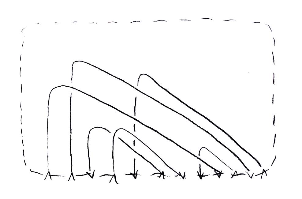
Let string A,B,C be given such that A and B cross C. Since there are no unnecessary crossings, if A and B do not cross, C will cross them in the order it has to. Assume A and B do cross, and let a,b,c be the boundary crossings A,B,C come straight out of respectively. Assume a<b. If a<c and b<c, then B crosses A when it comes straight out of b, so B will arc down above A, so C will cross A closer to c than B. If a<c and c<b, then C will cross A when it comes straight up from c, then it will cross B when B comes straight up from B, so still A crosses closer to c than B. Finally, if c<a and c<b, A will cross C when it comes straight up from a, then B will cross C when it comes straight up from b, so again A crosses C closer to c than B. Hence it is possible to position any simple weave in standard form. ∎
Usng this theorem, a simple weave can be represented by a map of inputs to outputs. All the crossings of the weave and their positions can be deduced from this by assuming the weave is in standard form. Not only is this a much more compact representation than an actual model of the boundary and the crossings in the weave, it makes comparing two simple weaves trivial. There are a number of other advantages as well, which will be pointed out later.
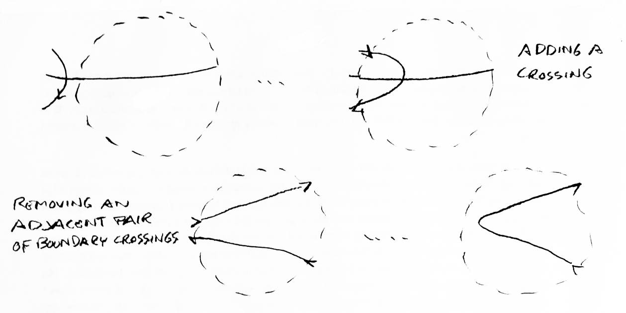
As noted before, links are actually special cases of weaves. The process of replacing a given weave with a set of simple weaves can be at least as expensive as finding the Homfly polynomial for links. This problem can be largely avoided by being very selective about what weaves you allow to occur in the first place. The algorithm is already deciding, before it even touches weaves, what order the crossings of the link are to be added to the solved region, thus how the boundary of each weave is going to be changed. These changes in boundary are what produce weaves which aren't simple. By changing the boundary in the smallest steps possible, replacing all weaves with simple weaves between every step, we can assure that the formula trees needed to replace weaves will be small.
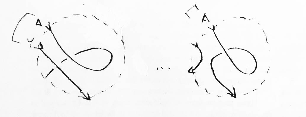
Adding a crossing to the solved region can be broken into two operations — adding a crossing which is only connected by one link, then two by two, removing crossings of the boundary which are adjacent and connected by an arc in the solved region (see Figure 27). Adding a crossing connected by one arc would then take one step, while one connected by two arcs would take two steps (adding a crossing and removing a pair of boundary crossings). Adding a crossing connected by three arcs would take three operations (one added crossing, two pairs of boundary crossings to be removed).
Note that this analysis of how the boundary of the solved region changes is all that needs to be known about the original link. Before any weave is touched, all the ways the boundary will change can be computed. Once a list of changes has been made, there is no need to refer to the original link. Also, once all these changes are known, the maximum size weave needed will be known, and a fairly accurate estimate of the time needed to compute the polynomial can be made easily. This modularization of the problem was unexpected, but it was a nice result.
Proposition: Adding a crossing to a simple weave which is connected to the weave by only one arc produces a weave that can be replaced by simple weaves with at most one application of the Homfly formula.
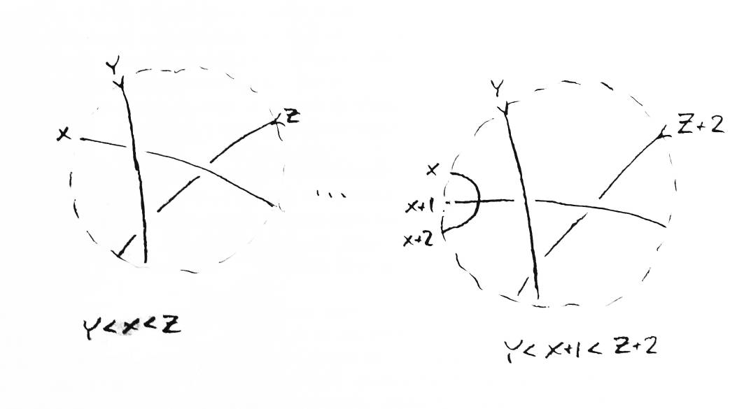
Proof: let P, a simple weave of n strings, be given. Consider adding a crossing connected to it by one arc at boundary crossing x (see Figure 28). This will produce a new string that crosses the old string at the crossing that was added. New boundary crossing numbers will be assigned. The new string will have number x and x+2 and the old will be renumbered as x+1. If the added crossing (the old string crossing the new string) is OK, you have a simple weave and you're done. Otherwise, the Homfly formula needs to be applied once. The switch will produce a weave that is OK. The break will reconnect the old string to either boundary crossing x or x+2. If x+1 is an output, no inputs have been moved, so you have a simple weave. If x+1 is an input, then the break from the Homfly formula reconnected the strings so the new string doesn't cross anything and the old one crosses what it did before the crossing was added. All inputs that were numbered below x before the crossing was added are still numbered below x, and all those numbered above are now numbered above x+2. Hence all crossings are still correct, and the weave is simple. Only one applicating of the Homfly formula, at most, was necessary to reduce the weave to a set of simple weaves. ∎
Proposition: Removing a pair of boundary crossings from a simple weave in standard form produces a free string if and only if the boundary crossings are connected inside the weave by a string, and the string crosses nothing.
Proof: A string connecting two adjacent boundary crossings does not need to cross anything. Since simple weaves in standard form have no unnecessary crossings, that means the string connecting them does not cross anything. If two boundary crossings are not connected by a string, then removing the boundary crossings simply connects two strings. Their other boundary crossings still exist, so no free string was produced. ∎
The case that this proposition deal with, where a free string is produced, is easy to test for. It requires no applications of the Homfly formula (the weave can be replaced by just one simple weave), but it does require multiplying the tag for the resulting weave by M-1(-L-1-L). The next section will show that this is the only case in which a free string needs to be produced when replacing a weave with a set of simple weaves (assuming the weaves being replaced were produced by one of our two boundary manipulations).
Let a simple weave P on n strings be given. Let u,v be adjacent boundary crossings in P which can be connected and removed. Note that u and v might be 0 and 2n-1, as these two boundary crossings are adjacent. Since the number of inputs and outputs in any weave are the same, either u is an input and v is an output, or vice versa. Let P' be the weave obtained by connecting and removing u,v from the boundary of P. For convenience, leave the boundary crossings in P' numbered the same as in P. Let A be the string of P' which is the union of the strings that used to end in u and v Let a be the input of A, and let z be either u or v, whichever was the input (see Figure 29). The part of A which used to be the string with input z will be called the tail of A. The rest will be called the head of A. A crossing in P' is bad if the input of the overpass is larger than the input of the underpass. All bad crossings in P will be in the tail of A.
Standard form and our method for determining overpasses are symmetric with respect to the numbering. The mirror image of a simple weave of n strings in standard form, with boundary crossings renumbered with i now 2n-1-i, is itself a simple weave in standard form. Hence we may assume, without loss of generality, that a < z.
Let B be the string in P' with the lowest (highest) input, b such that b<a<z (or a<z <b). In every crossing that B is involved in, B is the overpass (underpass). Consider the boundary of P' as a cylinder. B lies entirely above (below) every other string, including A. An application of the Homfly formula to a bad crossing, causing a switch and a break, would mess with strings in the vertical region between the two strings the operation was done on. Therefore no sequence of applications of the Homfly formula to bad crossings could produce a weave in which B has a bad crossing. Inductively, we find that the only strings that we can mess with are those with inputs between a and the highest input which currently has a bad crossing.
Let Y be the string with the highest input in P which currently has a bad crossing. Y crosses the tail of A s an overpass. It might cross the head of A as well, but there it would correctly be an underpass. By applying the Homfly polynomial to the bad crossing of Y, we get two weaves (the switch and the break).
Consider the break. No free string is produced. Y replaces the part of its string following the bad crossing with the part of the tail of A following the bad crossing (see Figure 30). Since the tail of A was originally a string with a higher input than y, and since Y is the string with the highest input that was capable of having a bad crossing, the new Y passes under every other string capable of having a bad crossing (which is correct) and is correctly an underpass or overpass for every string that was incapable of getting bad crossings. The new Y will cross itself at most twice (see the lemma below), so Y will not be knotted. Hence there are no bad crossings in the new Y. Also, Y's input is now higher than the input of the highest string with bad crossings, so Y will never be given any more bad crossings. All the bad crossings in the break are in the new tail of Y.
In the switch, either Y now has no bad crossings, or you shouldn't have applied the formula in the first place — do a Type II Reidemeister move to remove both bad crossings. Either way, Y now has no bad crossings and is incapable of being given any because it now has an input higher than the highest input with a bad crossing. All the bad crossings are in the new tail of A. Repeat this method, getting rid of the bad crossings of the highest input wtih bad crossings, on the switch and the break until all resulting weaves are simple. Since each step produces a string that does not need to be considered, the formula stree will have a depth no greater than n-2 (minus one for combining two strings to produce A, minus one because A crossing A doesn't count). Since no string crosses itself more than twice (see the lemma below), no string is knotted, so no more crossings need to be considered. Hence a weave (formed by removing a pair of boundary crossings from a simple weave) can be replaced with a set of simple weaves in 2n-2 steps.
Lemma: When replacing a weave of the type described above with a set of simple weaves by the method described above, A will never cross any string that can have bad crossings (including itself) more than twice.
Proof: (see Figure 31) (There are too many cases here to handle individually. Pictures of all cases are given.) Originally, A is in one of these four shapes (ignoring the string that can't be given bad crossings). All the types of strings that cross A and can have bad crossigns are shown. Only breaks can change the shape of A (switches just remove strings from consideration). In most cases, the break rotates the tail of A clockwise. In the shapes where the output of A (call it x) is between a and z, the strings with inputs between a and x won't be touched until all those between x and z are taken care of. Once they can no longer get bad crossings, a break wouldn't really change the shape of the string (see Figure 32). Hence breaks will make A stay in these shapes. Also, there is no break that would cause a string other than A to cross itself. ∎
If adding a crossing x to a weave is lumped with the first removal of a pair of boundary crossings from W+x (see Figure 33), a set of simple weaves replacing it can be found in (2)(2n-2) = 2n-1 applications of the Homfly formula. This keeps the largest weave that needs to be considered for a link of c crossings down to ⌈√c⌉, rather than ⌈√c⌉+1 (which it would have to be if you added a 2-connected crossing as first a one connected one, then removed a pair of boundary crossings). Also, there are quite a few weaves where you can tell from how inputs and outputs are matched that no more than one application of the Homfly polynomial will be necessary to replace the weave with a set of simple weaves. Experimental evidence shows this is the case with about 70% of the weaves that are encountered. Representing simple weaves as a matching of inputs to outputs lets these weaves be picked out immediately, without needing to actually model their strings.
We have seen that the Homfly polynomial for a link of c crossings can be computed using sets of no more than n! simple weaves, where n is ⌈√c⌉. What is the best way of picking out duplicates of weaves when they occur, so their polynomials can be summed and only one copy of the weave need be kept? The fact that simple weaves can be represented by the way their inputs are matched to their outputs again comes to our aid. This matching can be seen as a permutation, and there is a total ordering on permutations. Experimental evidence shows that usually between a sixth and a half of all possible weaves of n strings are actually used by this algorithm. The weaves can be stored in an array, where the index to the array is determined by the permutation representing the weave and by the total ordering of permutations.
Two orders of the strings of a given weave were used by this algorithm: the order determined by the inputs (used for representing the string and for determining overpasses), and the order determined by the smallest boundary crossing (used to put weaves in standard form). The order determined by the smallest boundary crossings can be represented as a list of higher boundary crossings they map to, but the numbers vary and the result can't be used to determine an index to the array of weaves. Well, it can, but only by converting it to the order of inputs first. Since neither order filled all the needs of this algorithm, I used both.
Let a link with c crossings be given. We have seen that an ordering of its crossings exists so that, as they are added to the solved region, weaves of size greater than ⌈√c⌉ (call this n) are never required. We have seen that all changes that need to be made to the boundary of the solved region can be determined before any weave is ever touched. We have seen that adding a crossings takes at most one application of the Homfly formula, and that removing a pair of boundary crossings takes at most 2n-2 applications of the Homfly formula. We have seen that no more than n! simple weaves are needed to represent the solved region at any time. Therefore the Homfly polynomial for a link can be computed in O(c(n!)(2n-1)) time, where n is the number of strings in the largest weave considered and n ist at most ⌈√c⌉.
This algorithm, specifically the first step in which a solved region with a small separator eats up a link, can easily be generalized to computing the other polynomial invariants on links, and with very little imagination can be generalized to problems like finding a Hamltonian cycle and other NP-complete problems on planar graphs. The characteristc of this algorithm that makes it different from most algorithms using graph separators is that it is not a divide and conquer strategy. The strategy is to make small changes, and to rely on quickly accomodating those changes and collecting resulting duplications. I believe a divide and conquer strategy would not work for computing the Homfly polynomial — at the first step, you would have two n-string weaves meshing with each other, forming (n!)2 combinations. That's the square of the order of this algorithm.
| [1] | K. Reidemeister. Knotentheorie. Julius Springer, Berlin, 1932. |
| [2] | Ralph. H. Fox and Richard. H. Crowell. Introduction to knot theory. Boston, Ginn, 1963. |
| [3] | Joan Birman. Annals of Mathematics Studies. Volume 82: Braids, Links, and Mapping Class Groups. Princeton University Press, 1975 |
| [4] | C McA. Gordon. Some Aspects of Classical Knot Theory. In Knot Theory, pages 1-60. Springer-Verlag, 1977. |
| [5] | John Russell Gilbert. Graph Separator Theorems and Sparse Gaussian Elimination. PhD thesis, Stanford University, December, 1980. |
| [6] | W. B. R. Lickorish. Prime Knots and Tangles. Transactions of the American Mathematical Society 267:321-332, 1981. |
| [7] | Louis Kauffman. Mathematical Notes. Volume 30: Formal Knot Theory. Princeton University Press, 1983. |
| [8] | P.Freyd, D.Yetter; J.Hoste; W.B.R.Lickorish, K.Millett; and
A.Ocneanu. A New Polynomial Invariant of Knots and Links Bullettin of the American Mathematical Society 12(2):239-246, April, 1985 |
| [9] | W. B. R. Lickorish and K. C. Millett. The New Polynomial Invariants of Knots and Links. Mathematics Magazine 61(1):3-23, February, 1988 |